
Demand planning is the process of predicting future demand and translating it into decisions for procurement, production, and inventory. A resilient demand planning framework rests on four design principles: the right forecasting models, the right granularity, planning horizons that match business needs, and KPIs that prove whether each process step actually adds value. This article walks through all four – including a comparison of demand planning models from classical statistics to machine learning, and the operating model that ties them together.
The starting point is familiar to most planning teams: more sales channels than ever, shorter product lifecycles, frequent promotions and new product introductions, and demand volatility that has become a permanent condition rather than an exception. Frameworks designed for stable demand quietly fail under these conditions – not with a bang, but through creeping forecast errors that materialize as excess stock on one shelf and lost sales on the next.
What Is the Demand Planning Function?
The demand planning function sits between the market-facing side of the business (sales, marketing, product management) and the supply side (procurement, production, logistics). Its job is to consolidate demand signals into one agreed forecast – a single source of truth – and hand it to supply processes in the granularity they need. Demand planning and demand forecasting are related but not identical: forecasting is the statistical prediction itself; demand planning is the end-to-end process around it, including inputs, review, consensus, and hand-over to supply planning.
Demand Planning Models: Statistical Methods vs. Machine Learning
The choice of forecasting model is the most visible design decision – and the one where the state of the art has moved fastest. An overview of the main model families and when to use them:
- Exponential smoothing (e.g. Holt-Winters): simple, robust, and interpretable – the right baseline for stable seasonality and rich sales history.
- ARIMA & Bayesian methods (e.g. SARIMA, BSTS): handle trend changes and prior knowledge well – suited for volatile demand and limited history.
- Intermittent-demand methods (e.g. Croston, SBA): built for sporadic demand patterns – the standard for spare parts and slow movers.
- Machine learning (e.g. gradient boosting with LightGBM or XGBoost): learns across the whole assortment and uses external features – best for large assortments, promotions, and external demand drivers.
- Foundation models (transformer-based time series models): transfer patterns learned from millions of series – strongest for new products without history and cold starts.
Classical methods analyze the structure of a single time series – trend, seasonality, residuals – and extrapolate it. They remain a solid baseline where patterns are stable. Their shared limitation: they see only one series at a time, with no cross-learning between products and no external demand drivers.
Machine learning models changed exactly that. Gradient boosting algorithms learn across the entire assortment and process arbitrary features – price, promotions, channel, weather, calendar effects – and have dominated forecasting benchmarks since the M5 competition [1]. Transformer-based foundation models for time series go one step further and transfer demand patterns learned from millions of external series onto your assortment, which is particularly valuable for new product introductions with no history. And reinforcement learning reframes the problem entirely: instead of optimizing the forecast as an end in itself, it optimizes the decision that follows from it.
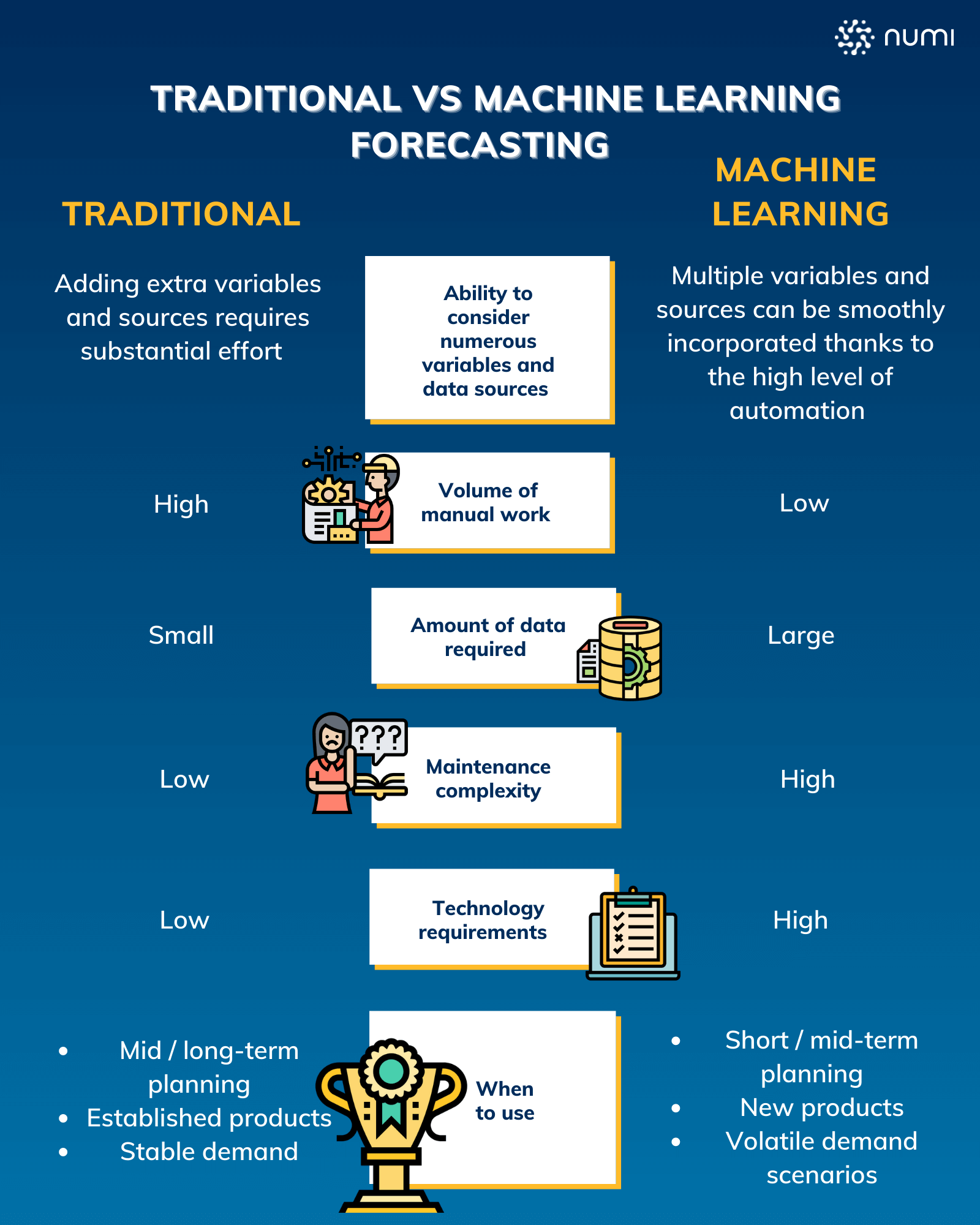
In practice, no single model wins for every product. Robust systems run ensembles: for each item, automated backtesting selects the model (or combination) that would have performed best over recent periods – continuously re-evaluated. A modern demand forecasting software handles this model selection, feature engineering, and retraining automatically. At refurbed, AI forecasting methods combined with external data sources reached 66% forecast accuracy and cut lost sales by 64%; across our customer base we see up to 35% higher forecast accuracy compared to the previous process.
Forecasting Granularity
The second design principle is the level of granularity. There are two perspectives: demand-driven (customer, channel, region) and supply- or product-driven (item, product group, location). The guiding questions: Who is the recipient of the forecast? And does a finer forecast hierarchy add measurable accuracy – or is a more aggregated level with far less effort sufficient?
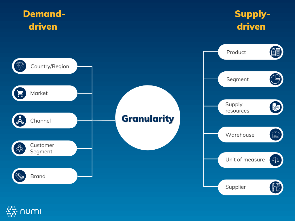
As a rule of thumb, aggregated forecasts are more accurate than granular ones – but only the granularity the recipient actually needs is operationally useful. A highly accurate monthly forecast at product-group level does not help a replenishment planner who orders items per warehouse. Recent demand volatility calls for more granularity rather than more aggregation; what matters most is the ability to aggregate and disaggregate consistently between hierarchy levels, so that strategic and operational decisions run on the same numbers.
Planning Horizons and Time Buckets
Forecast horizon and time aggregation should follow the recipient and the process lead times, not habit. Annual financial forecasts do not need weekly buckets; operational forecasts for warehousing or transportation require daily buckets or order-level granularity. For fast-moving goods with a seven-day replenishment lead time, an eight-to-twelve-week horizon is sufficient. Long raw material sourcing from Asia with complex manufacturing requires a one-to-two-year horizon to plan supply capacity.
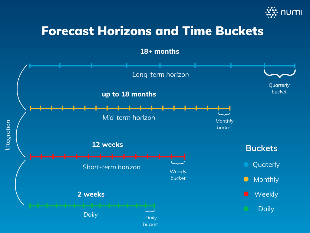
A typical hidden error source: KPIs measured on a different horizon or bucket than the one the forecast is operationally used on. A forecast that looks solid at monthly level can be unusable at weekly level. The trend is clearly toward more frequent, more granular planning cycles – weekly instead of monthly cycles catch demand shifts earlier and prevent bias from accumulating.
Demand Planning KPIs and Forecast Value Add
Improvement starts with measurement. The choice of metric strongly influences the outcome: RMSE overweights outliers, an isolated MAE hides systematic bias. A combination is therefore standard – an accuracy metric plus forecast bias, which shows whether you systematically over- or under-forecast and is usually the fastest indicator of a misconfigured process.
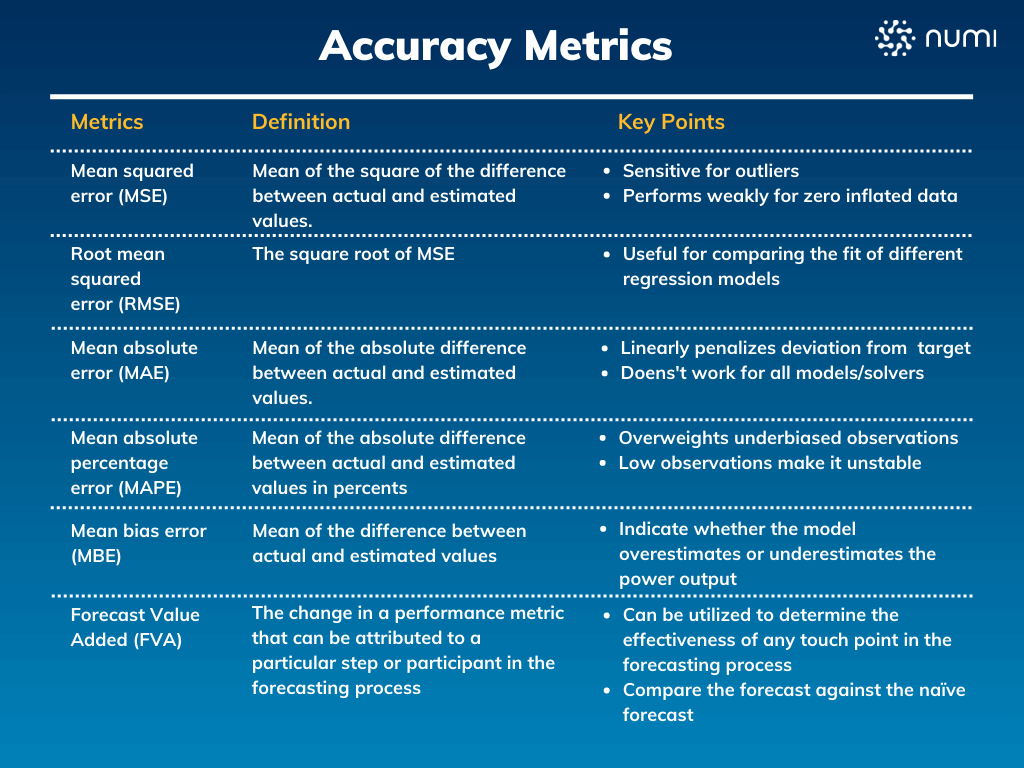
The second essential metric is Forecast Value Add (FVA): it tests whether a method, an additional input, or a manual override actually improves on a naïve reference forecast. The results are often sobering – a substantial share of manual overrides makes forecasts worse. FVA makes visible which process steps earn their effort and which only add noise. A full overview of the metrics, including formulas, is available in our article on forecast KPIs.
The Demand Planning Target Operating Model
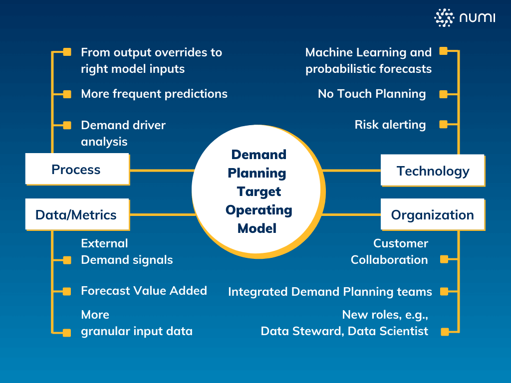
The design principles above need to be embedded into a process enabled by the right technology and organizational setup. The target picture of modern demand planning is "no-touch": models generate, monitor, and update forecasts automatically; planners intervene only where they demonstrably add value, steered by exception alerts instead of clicking through thousands of items. This improves accuracy twice over – models are refreshed far more often than any manual process allows, and the FVA-negative share of manual overrides disappears.
Instead of building a baseline forecast and having sales, marketing, and product management enrich it manually, their information – promotions, CRM signals, new product plans – enters the model directly as structured inputs, alongside external data like point-of-sale, IoT, and market signals. The next step is already visible: AI agents that derive and execute decisions from forecasts automatically – from purchase order creation to supplier communication. Forecast accuracy remains the foundation, but the competitive edge is shifting to how fast a forecast becomes a decision.
Organizationally, this means clear forecast ownership, data quality as an explicit role (data steward), and seamless hand-overs to logistics, production, and procurement – without manual interfaces where accuracy gets lost. External partners such as key customers can contribute demand signals directly; in some setups a jointly maintained demand plan is worth the coordination effort.
Frequently Asked Questions
What are demand planning models? Demand planning models are the forecasting methods used to predict future demand – ranging from statistical time series methods (exponential smoothing, ARIMA) and intermittent-demand methods (Croston) to machine learning models (gradient boosting) and transformer-based foundation models. Modern systems combine them in ensembles and select the best model per item through automated backtesting.
What is the demand planning process? The demand planning process consolidates demand signals from sales, marketing, and product management into one agreed forecast, enriches it with statistical and external inputs, measures its quality with KPIs such as MAPE, bias, and Forecast Value Add, and hands it over to supply planning in the required granularity and horizon.
What is the difference between demand planning and forecasting? Forecasting is the statistical prediction of future demand. Demand planning is the broader end-to-end process around it: gathering inputs, generating and reviewing the forecast, building consensus across stakeholders, and translating the result into supply decisions.
How accurate should a demand forecast be? It depends on granularity, horizon, and assortment volatility. At item-week level, 60–80% accuracy (1 − WMAPE) is a realistic corridor; aggregated monthly levels reach significantly more. More important than the absolute number is the trend over time and the comparison against a naïve baseline (FVA).
Want to see how much forecast accuracy is hidden in your data? Book an intro call – we will show you, based on your own sales history.
Sources:
- https://www.kaggle.com/c/m5-forecasting-accuracy
- https://en.wikipedia.org/wiki/Exponential_smoothing
- https://en.wikipedia.org/wiki/Gradient_boosting